Microsoft Tips >>>
Adding a Dynamic Graph to Excel
I work a lot with large data sets in Excel, which are largely data sets for specific dates. One of the things I have wanted to do for a long time, is to make it so that I can display the data in a dynamic graph, and by that I mean to be able to specify the date ranges of data to use in the graph dynamically.
What I discovered was the OFFSET function, and after a lot of experimentation I have finally managed to work out how to get it to work, the following documents the process that I use.
Identify The Data Set
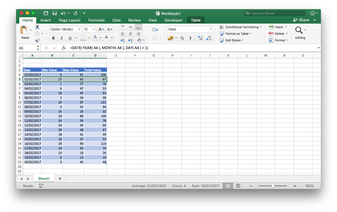
Firstly you need a set of data to create the dynamic graph against, I will use a sample set for the purpose of this demo and for simplicities sake have created this in a table in the spreadsheet with the following formulas
| Date | Min Value | Max Value | Total Value |
|---|---|---|---|
| 01-02-2017 | =RANDBETWEEN(1,20) | =RANDBETWEEN([@[Min Value]],100) | =[@[Min Value]]+[@[Max Value]] |
| =DATE(YEAR(A4),MONTH(A4),DAY(A4)+1) | =RANDBETWEEN(1,20) | =RANDBETWEEN([@[Min Value]],100) | =[@[Min Value]]+[@[Max Value]] |
Create the Default Graph
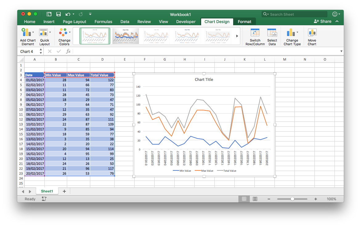
Next we add a Line Graph to the page

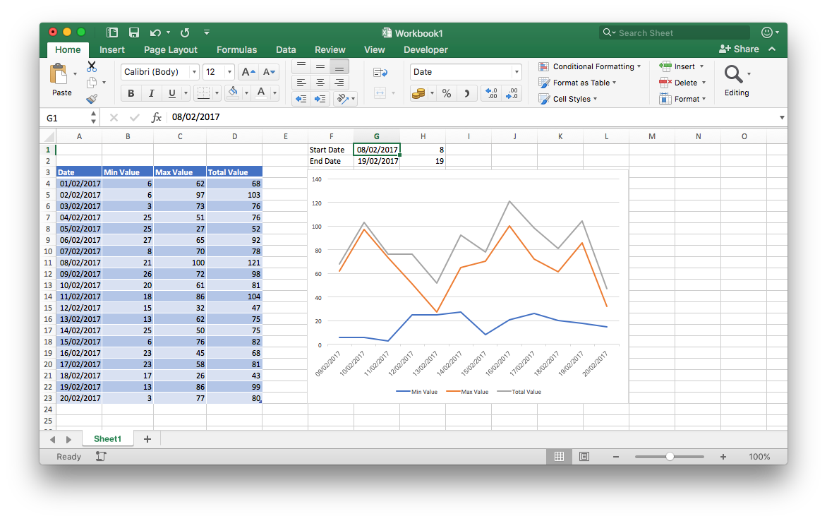
And the data series is automatically picked up from the table and you should have something like this
Make it Dynamic
But what I want to do is to allow the graph to be changed dynamically, so here are the steps that will facilitate that.
Step 1
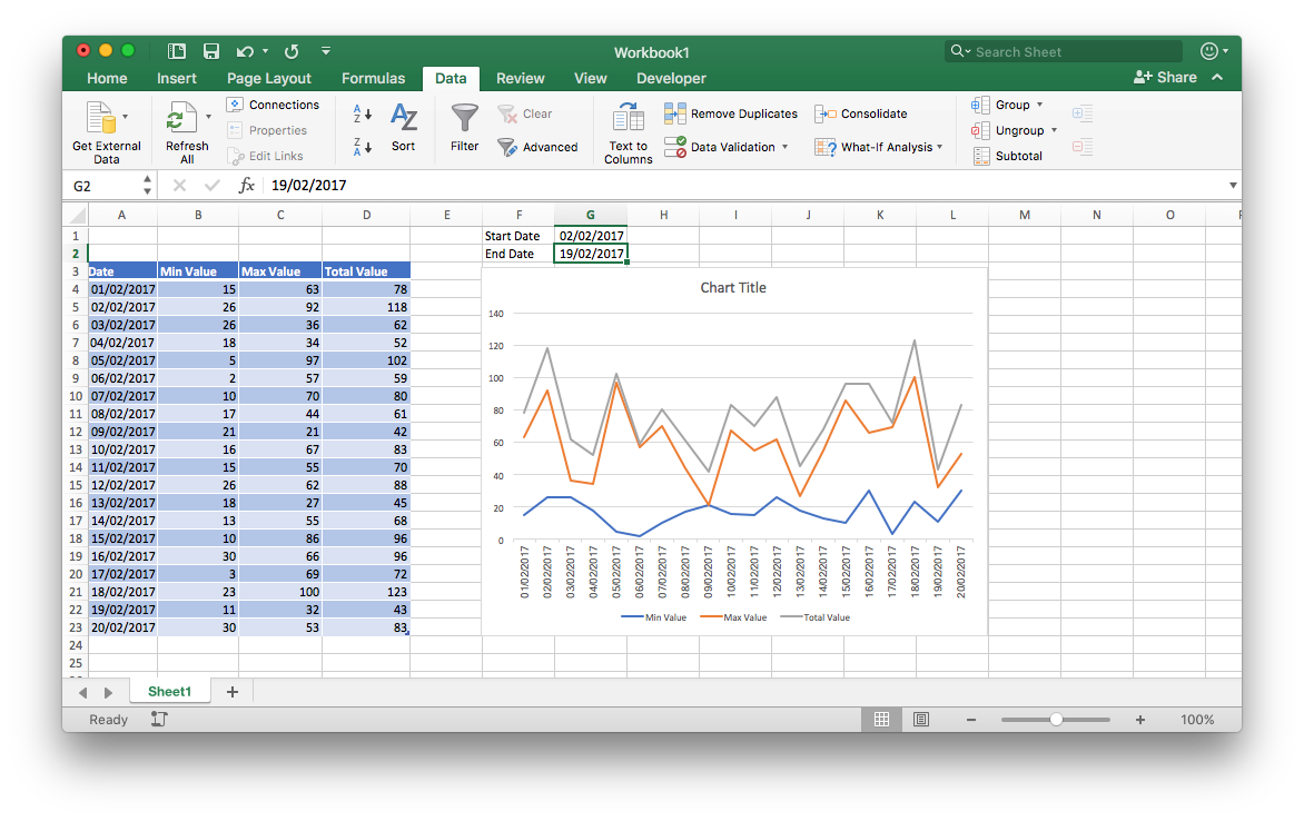
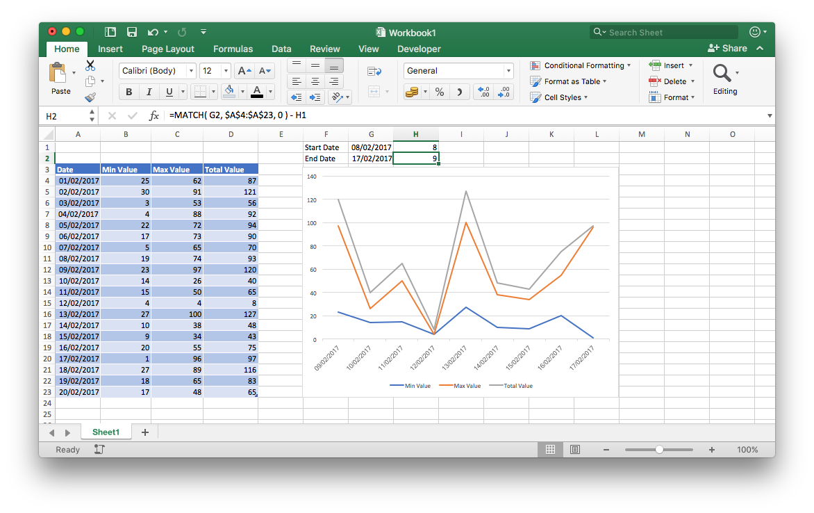
Add a couple of fields above the chart to hold the desired start and end date
NOTE: You must set the format of these fields and populate them before completing the validation steps below
Step 2
Add some data validation to make sure that we don’t break the graph by adding invalid data
On the Start Date field add the following Data Vallidation formula: This will force the Start Date to be between the min and max in the table, and less than the value entered in the End Date
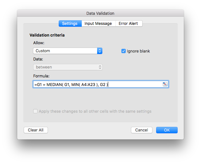
On the End Date field add the following Data Vallidation formula: This will force the End Date to be between the min and max in the table, and greater than the value entered in the Start Date

Step 3
To make this all work we use a little know feature know as OFFSET and the first part of this is to create a lookup value from the start and end data fields.
Add the following formulas to the Start and End Date fields
In the Start Date field enter the following formula
=MATCH( G1, $A$4:$A$23, 0 )

In the End Date field enter the following formula
=MATCH( G2, $A$4:$A$23, 0 ) - H1
Later on I will set these fields to have white text so we cant see it, but for now it helps to see what is going on
Step 4
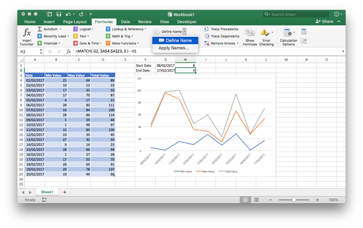
The clever part of this process is to create some Data Ranges using the OFFSET command, and this is done from the Formula tab by selecting the Define Name option as shown below
Step 5
It will help if you understand what the OFFSET command is doing rather than just blindly following my commands, so for those who are interested the definition of OFFSET is replicated from the Microsoft Website below
Description
Returns a reference to a range that is a specified number of rows and columns from a cell or range of cells. The reference that is returned can be a single cell or a range of cells. You can specify the number of rows and the number of columns to be returned.
Syntax
OFFSET(reference, rows, cols, [height], [width])
The OFFSET function syntax has the following arguments:
| • | Reference: | Required: | The reference from which you want to base the offset. Reference must refer to a cell or range of adjacent cells; otherwise, OFFSET returns the #VALUE! error value |
| • | Rows: | Required: | The number of rows, up or down, that you want the upper-left cell to refer to. Using 5 as the rows argument specifies that the upper-left cell in the reference is five rows below reference. Rows can be positive (which means below the starting reference) or negative (which means above the starting reference) |
| • | Cols: | Required: | The number of columns, to the left or right, that you want the upper-left cell of the result to refer to. Using 5 as the cols argument specifies that the upper-left cell in the reference is five columns to the right of reference. Cols can be positive (which means to the right of the starting reference) or negative (which means to the left of the starting reference) On |
| • | Height: | Optional: | The height, in number of rows, that you want the returned reference to be. Height must be a positive number |
| • | Width: | Optional: | The width, in number of columns, that you want the returned reference to be. Width must be a positive number |
Step 6
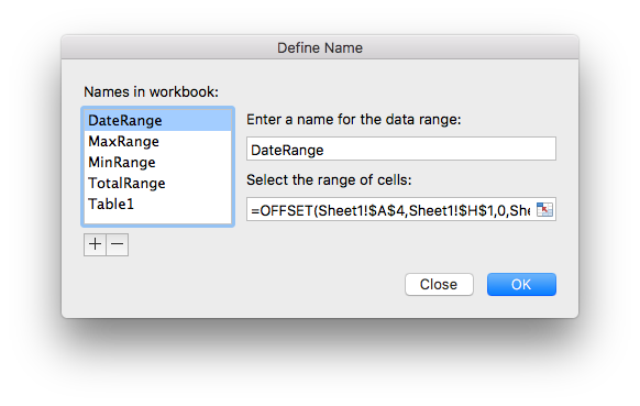
Armed with the information create the following 4 Data Ranges
| Enter a name for the data range: | select the range of cells |
|---|---|
| DateRange | =OFFSET(Sheet1!$A$4,Sheet1!$H$1,0,Sheet1!$H$2) |
| MinRange | =OFFSET(Sheet1!BA$4,Sheet1!$H$1,0,Sheet1!$H$2) |
| MaxRange | =OFFSET(Sheet1!$C$4,Sheet1!$H$1,0,Sheet1!$H$2) |
| TotalRange | =OFFSET(Sheet1!$D$4,Sheet1!$H$1,0,Sheet1!$H$2) |
You should end up with something that looks like this
Step 7
Now to put it all together
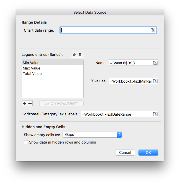
Go back to the graph and select the Chart Design Tab, then the Select Data Option then make the following changes
Set the Horizontal (Category) axis labels:  =Workbook1.xlsx!DateRange
Set the Min Value Y values:                 =Workbook1.xlsx!MinRange
Set the Max Value Y values:                 =Workbook1.xlsx!MaxRange
Set the total Value Y values:               =Workbook1.xlsx!TotalRange
Completed Dynamic Graph
Thats it, test away

Use this link to download the sample file