<<< Microsoft Tips >>>
Using 3D Arrays in Excel
I work a lot with large data sets in Excel, and have a number of tools that allow me to select a product type and have the price and currency auto populate through the pricing pages of he spreadsheet.
Until recently I used to use HLookup and VLookup to perform these tasks, but these two function have a number of undesireable features, not the least of which is that the data sets have to be ordered before the functions will work properly.
What I needed was something with much greater flexibility, what I found was INDEX and MATCH.
This page documents how to get these two functions to perform a much more satisfactory array lookup
Identify The Data Set
Firstly you need a set of data to create the lookup against, I will use a sample set for the purpose of this demo and have replicated that data in the table below which you can copy into a spreadsheet, allowing you to follow this demo.
| Product | Small Rack | Medium Rack | Large Rack | |||
|---|---|---|---|---|---|---|
| Oracle SuperCluster | $ | 375,000.00 | $ | 652,000.00 | $ | 1,067,000.00 |
| Oracle Exadata | $ | 330,000.00 | $ | 602,000.00 | $ | 1,098,000.00 |
| Oracle Exalogic | $ | 370,000.00 | $ | 600,000.00 | $ | 1,035,000.00 |
| Oracle Database Appliance | $ | 18,000.00 | $ | 24,000.00 | $ | 40,000.00 |
| Oracle Compute Cloud Service | $ | 50,000.00 | $ | 81,000.00 | $ | 114,000.00 |
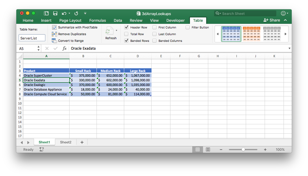
I have used an Excel table to hold the data and named this ServerList, this will help us later on.
Create Some Lookup Cells
The whole point of this is that it is possible to select the product and size in two drop down lists and retrieve the price, very simplistic I know but this does demonstrate the use of the INDEX and MATCH functions in a way that VLOOKUP and HLOOKUP would struggle.
So the next step is to add two lookup cells to the spreadsheet.
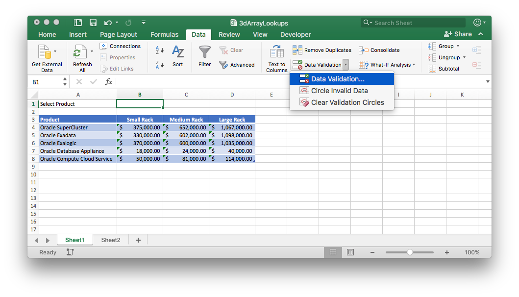
Step 1
Enter “Select Product” into cell A1, then from the cell B1, go to the Data tab and select Data Validation
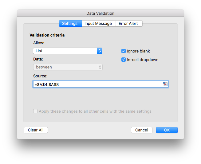
Step 2
Choose List as the Validation criteria and set the source to be the Product values from the table
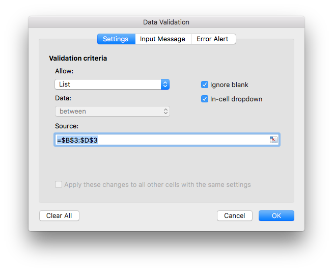
Step 3
Repeat this process in Cell A2, except this time enter “Select Size” into the cell and set the source to be the Table Headings
NOTE: we only want the Small - Large values in the drop down
Step 4
The final step is to bring this all together by adding the text “Cost of Product” into Cell C2 and following formula into Cell D2, you might also find it helpful to set the formatting of cel D2 to Accounting
=INDEX( ServerList, MATCH( B1, ServerList[Product], 0 ), MATCH( B2, ServerList[#Headers], 0 ))
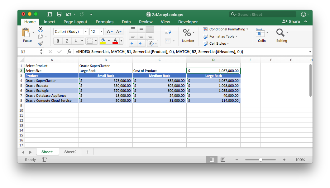
Now as you change the values in the two drop down lists the values in the Cost of Product Cell change to match the selection
Step 5
So how does it all work, I have included links to the Microsoft Website for both the MATCH function and INDEX function for those of you that are interested, otherwise there is a brief decription below.
Description
We are taking advantage of a couple of features here
- The INDEX function will return the value of an element in a table or array based on the row and column number provided. This is why we created a table as we can use the table name in the INDEX function.
- NOTE: that the rows and columns are all in reference to the top left corner of the array, and in our example you should have noticed that we only select the body of the table.
- The MATCH function searches for a specified item in a range of cells and then returns it’s relative position of that item in the range. This is why we created the drop down list from the array we are going to search.
- NOTE: it is imperative that we inform MATCH to use perform an exact match, which is what the 0 is for in the Match Command. If you don't you will get unexpected results and this becomes particularly important when you are performing numeric Matches.
- NOTE: you should have also noticed that the second MATCH string included the first column in the search, i.e. it included all of the headings, not just the ones we were searching for. This is because the INDEX function returns the values based on their relative positions and as we have searched the entire body of the table we needed to include the product column to return the correct value from the table array.
And thats it, test away